Context In a recent research report Heilig et al. [1] investigated various aspects of the effect of the ANN-outlier Panel replacement protocol with respect to its effect on the 95% Confidence Intervals of the ExcelÔ OLS-two parameter (Intercept:a and Slope: b) linear forecasting equation (OLSR). The ANN-protocol is an acronym for the Average of the Nearest Neighbor Points. Specifically, if the Panel of data under examination is:

Where,

ϵ represents an error of such a magnitude that 〖(x+ ϵ)〗_(t=k)  is identified as an outlier using a standard outlier screening protocol.

In this case, the ANN-replacement is:

H&L selected a Panel of 12 Time Series [TS] observations from 22 firms randomly selected from the Bloomberg^TM Markets platform and examined three ANN-replacements:

ANN: Replacement [Both [Early & Late]]: (x)_(t=2) & (x)_(t=11)

ANN: Replacement [Late]: The Next to Last Panel Point: (x)_(t=11)

ANN: Replacement [Early]: The Second Panel Point: (x)_(t=2)

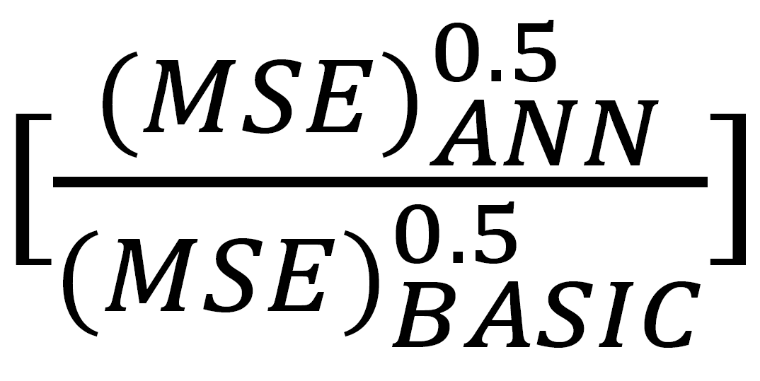
Their effect-variable of interest was the ratio:

Where,

presents the Precision of the 95%OLSR Confidence Interval and the (MSE)_•^0.5 is the root of the Mean Square Error[MSE] of the OLSR-fit for the Panel [·] under analysis.

If R_ANN is <1.0 the effect of the ANN-modification is labeled as: Smoothing as the OLSR-MSE-variation created by the ANN-modification decreased relative to the OLSR-MSE-variation of the BASIC unmodified series. Thus, smoothing produces a CI with smaller precision than was the case for the Basic Panel. Provoking is the designation for ratios >1.0 and No Effect is the label if the ratio = 1.0. H&L report of the 488 tests 314 were Smoothing or 64.3% (314/488). Further, they created a Screen, called the Comfort-Zone (CZ) for re-classifying the Smoothing or Provoking ratio-effects of ±2.5%: (97.5%; 102.5%) or (0.975; 1.025). Specifically, if the Smoothing ratio was <than 0.975 it was labeled as a Serious Smoothing Effect; for ratios >1.025 a Serious Provoking Effect was recorded. H&L note, in this CZ-calibration, there were 201 Serious-events and 173 were Smoothing: (Both 79 + Late 51 & Early 43) or 86.1% (173/201) Also see Table 2 (Panel: A: Col (RRP)) in this research report.

Details of the Research This Smoothing tendency presented by H&L was heretofore not reported in the peer-reviewed literature. For this reason, their Smoothing-study begs additional testing-arms. This is the point of departure of our re-analysis of their data. Specifically, we:

• Present a behavioral context that tacitly cajoles replacement of outliers

• Detail the essentials of the Time Series (TS) Regression Forecasting Model used to form the forecasts and the related 95% Confidence Intervals, 

• Extend and detail the TS-ANN Replacement Protocols used to create comparative ANN-information

• Discuss the Accrual of the Firms and their sensitive account Panel variables used to develop the TS-forecasts of the accounting data

• Offer various Vetting Tests, the intention of which, are to engender understanding and confidence in the meaning of inferences drawn from the various probability tests to be reported

• Detail Four variable measures sensitive to: Forecast & Precision Modification-Effects

• Present detailed Tabular Profiles of all the study impact variables and selected Inferential Illustrations that can be used by the readers to examine aspects of the modifications that would inform their decision needs

• Offer a Summary and an Extension of this study

The Behavior Context for Outliers

Overview The label “Outlier” has a pejorative linguistic connotation that all but requires the analyst to “take a corrective action”. The Merriam-Webster: definition of an outlier in a statistical context is:

A statistical observation that is markedly different in value from the others of the sample; values that are outliers give disproportionate weight to larger over smaller values.

This standard definition effectively “prods” the Decision-Maker (DM) to “do something about this problematic or troublesome data-point” that has “objectively” been labeled as an outlier. Thus, this interesting coupling of {Outlier & Corrective Action} has promoted the tendency to replace data in TS-Panels or at least compensate for them in the modeling process. In most standard texts, such as the one that we used in our forecasting course [2], there are advisories against making an inference where there are likely to be outliers in the dataset. For this reason, many forecasting and data-analytic software platforms offer a number of techniques for identification of outliers with the obvious intention to “deal with them in some acceptable manner”. For example, the SASÒ [3],, publication: Econometrics and Time Series Analyses in the Regression Section notes regarding options for this analytic platform:

Specify Outlier Options

Enables you to control the reporting of Additive Outliers (AO) and Level Shifts (LS) in the response series.

Additionally, SAS has a model that can be used to “tease out” the effect of possible outliers called: Recursive PartitioningÓ based upon elimination or re-positing model parameters.

Usually, outliers are identified using an outlier-screening platform. The “gold-standard” screening protocol is the Box-Plot [4], where points outside of the whiskers are designated as outliers thus, all but requiring, that an action be taken. Further, the SAS/JMP® Statistics and Graphics Guide [5], lists the Histogram, Normal Quantile Plot, Quantile Box-PlotÓ and the Stem & LeafÓ as possible outlier-screens.

Focus of this research report: Testing the ANN-effects as context, it was detailed above that there:

• Is a linguistic behavioral “imperative” for analysts to correct for outliers

• Is a plethora of outlier screening platforms, the use of which is synonymous with best practices in creating meaningful forecasts and/or data-analytic recommendations in the Audit context

• Are numerous analytic-platforms that have output conditioning platforms to adjust for outliers

These three features combined with “a” conventional wisdom in the practicing forecasting community that replacing outliers is:

• Critical usually true

• If one uses Simple and Logical replacement protocols that this mode d’emploi would enhance the information content of the forecast

The principal support for this logical-montage is that Simple and Logical replacement protocols are robust–to wit: They would have No Material Effect on forecasts drawn from the basic Panel IF there were to be no actual outliers. Thus, such protocols would be harmless if used when not needed and so can only be useful. This concept, as it pertains to Outlier-Protocols is best characterized as Robust–in–Utility.

Given this preamble that borders on a homily, we should expect that an extended study that addresses the impact of replacement of outliers would be of practical value to the practice of forecasting. Such a study could be a base-line for the Missing Data Panel replacement protocols in a time-series context. Thus, the focus of this research extension is to address the presumed Robustness-in-Utility of the ANN-Protocol. In this regard, we will:

Investigate the effects of ANN-replacements for: 

• Meaningful and sensitive forecasting variables composed of {Forecasts & Precisions}

• Varying Panel-lengths

• Examining the symmetry of these ANN-effects

• Vetting the “2 to 1”-Smoothing percentage reported by H&L

The Forecasting Model

To generate a forecast Ŷₜ we will use the Excel™ Platform (Data Analysis Regression). This form will be the OLS-two parameter linear (Intercept & Slope Trend) Time Series Regression model (OLSR) used to forecast from a TS-Panel. In the TS-version, the dependent variable is the traditional Y-variate (Ordinate) and the integer Time Index is the equally spaced independent-variate [Abscissa] where: the first point X_t=0 is indexed as 1 and subsequent points follow as integers to the last point all of which are used in the OLS-fitting. 

OLSR Inference from the Excel Parameter Range Model the Excel Regression functionality (Data (Data Analysis (Regression) forms a “wide-covering” confidence interval for the one-period ahead forecasts compared to the Fixed- or Random- Effects projections [6]. For this reason, we are NOT interested in the capture-rate of these Excel 95%CIs; almost certainly, these wide-95%CIs will capture most of one-period-ahead holdbacks. We are forming these 95%CIs as they will be used in the creation of sensitive test variables; and also, the ratio of the precisions of 95% CIs is the ratio of the OLSR-Standard Errors [σ^] and so is a simple measure for calibrating the effect of the ANN-modification Smoothing or Provoking.

Instructive Illustration It is usual to script an illustration to clarify these computations. This will be done using the data from the Hershey Corporation, Inc. (HSY) downloaded from the Bloomberg Markets™ platform.

For a one-period ahead forecast, h = 1, we produced the following information:

The TS-version of the 95%CIs for the HSY-dataset are:

Extreme Left Side (Lower-Limit 9LL)) 95% Boundary for the first projection horizon (h = 1) is:

Extreme Right Side (Upper-Limit (UL)) 95% Boundary for the first projection horizon (H1) is:

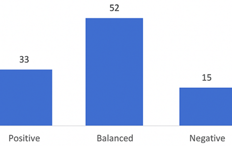
Using the usual definition of precision—i.e., 50% of the spanning-length of the confidence interval—the precision of this forecast is: 50% × (2,071.6 - 357.3) = 857.2. Note, as a computation-check, that the mid-point of the confidence interval is the forecast e.g., ((357.3 +2,071.6) /2) = 1,214.45. Finally the Mean Square Error (MSE) is 51,053.65 and so the Standard Error [ of the OLSR is: √51053.65 = 225.95.

Modification Protocols: The Account Base

Accounting Variable Set for Forecasting We used the exact same H&L-dataset so as to control for inter-test randomization effects. For each firm, we selected four Income Statement variables: {Gross Profit; Operating Income; Earnings for the Common Shareholders; Shares for Diluted Earnings per Share} and four Balance Sheet Statement variables: {Current Assets; Other Assets & Deferred Charges; Current Liabilities; Current Ratio}. For each of these eight accounts, we selected 12 data-points starting 2005:t₁ to 2016:t₁₂.

Panel Modifications Download Panel

No modifications: Baseline Panel [BP]: {x_(t=1), ..., x_(t=12)}. To test for the Panel-Length effect we created two variations from the BP (n = 12). The Mid-Length Panel (MP) was created by removing three Points: {x_(t=10), x_(t=11), x_(t=12)}  from the Download Panel:BP. MP (n = 9) is then: {x_(t=1), ..., x_(t=9)}. Finally, the Short-Length Panel (SP) removed three Points: {x_(t=7), x_(t=8), x_(t=9)}  from MP (n = 9). SP (n = 6) is thus: {x_(t=1), ..., x_(t=6)}. For each of these three Panels: {BP; MP & SP} datasets, we made the following three ANN-replacements.

ANN: Replacement (Early): The Second Panel Point: (x)_(t=2)

 Table 1: HSY Panel: Other Assets: Deferred Charges

ANN: Replacement (Late): The Next to Last Panel Point: (x)_t=(n-1)

ANN: Replacement (Both 9Early & Late) : (x)_t=2 &  (x)_t=(n-1)

Thus, there are nine-test-arms: 

BP (E: L: B), MP (E: L: B), SP (E: L: B)}

Nature of the Replacement Protocols

The critical questions of this research report are: For the ANN-protocol, what are the magnitude and nature of the effects relative to the BP likely to be? If the conventional wisdom of Robust-in-Utility, is correct re: the ANN-protocol, then there should be basically No or Unimportant effects relative to the BP to wit, inferentially the ANN-protocol will be Robust-in-Utility. The counter point thus is the H&L-research report where about two-thirds of the time the ANN-modifications created important Smoothing effects. As noted above, one of the test-foci of this research report is to vet the H&L indication of a Smoothing tendency.

Illustrative Profile

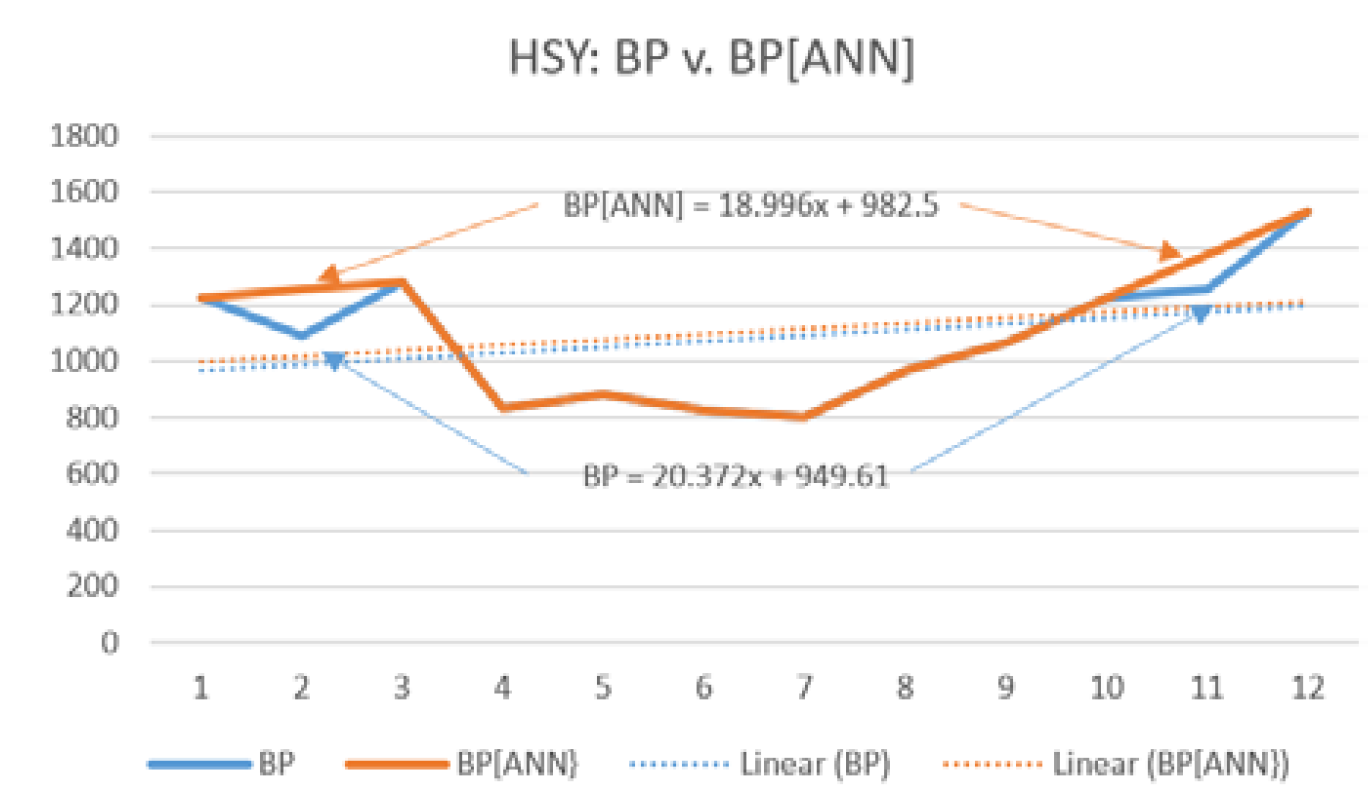
At this point, it would be useful to offer a graphical profile of the nature of the effects created by the ANN-protocol. For example, for the HSY-Panel (Table 1), we made the ANN (Both) transformation. Results: The BP[] was 225.9506 and the ANN: Both [] was 244.5366. This ratio: (ANN: Both []/BP[]) is 1.0823. This is, of course, also the ratio of the Precisions of the 95%CIs of the two series: (927.67/857.16). Thus we can reject that the ANN (Both) is, by nature, smoothing as 1.0823>1, this indicates that the BP (ANN (Both)) is Provoking (Figure 1).

The dashed lines are the OLSR: Excel regression-lines [- - -] of the BP and the BP (ANN). The graphic highlights the change at points n = 2 and n = 11 where the ANN[Both] modification was effected. Essentially, the transformation moved the transformed series “away” controlling for the OLSR-reorientation effected by the ANN, from the regression line of the BP series and this is why BP[] went from BP [] = 225.9506 to 244.5366 for the 

ANN: Both []. Specifically, the Both (ANN-transformation) shifted Point 2 and Point 11 away from the regression lines formed from the BP and the BP (ANN) datasets and overall the orientations resulted in an increase in the OLS-distance from the respective regression-line. However, the operative issue is also the magnitude of the Provoking-effect that will be consider subsequently. 

Figure 1: Plot of a Provoking Replacement

Testing Variables

The Inference Context: To develop informative profiles that address the forecasting and precision effects of the proposed ANN-replacement modifications BP, Both, Late & Early as well as the Small, Medium & Large blocking, we will create four variables in Sections 5.2, 5.3, 5.4 & 5,5. Additionally, to address the magnitude of possible effects of the ANN-Protocol we will re-calibrate the “Comfort-Zone” used by H&L.

Re-calibration of the H&L-version of the Comfort Zone (CZ) The logic of using a CZ-filter is to focus on “Events of Interest”. Rationale: In any measurement calibration in a forecasting context using accounting data from firms traded on active exchanges, there is stochastic variation that is generally labeled as “noise”. This being the case, event-measurements falling into this un-avoidable “noisy” stochastic-zone are of little analytic interest. To focus on Events of Interest, we have selected a band-width of 5% as this is also the usual calibration for the False Positive Error for the 95% non-directional level of confidence often used in most analytic contexts. Thus, our CZ-band will be noted as: ±2.5%CZ. H&L applied their CZ-version directly to the ratio:

in this research extension, we will use the ±2.5%CZ-screen with a sensitive benchmark for the variables that we will use in this study. Point of Information. In the H&L-version, the Left Hand Side (LHS) of the CZ indicated a Smoothing Event and Events in the Right Hand Side (RHS) were Provoking in Nature. In our re-calibration, there are still Smoothing and Provoking aspects but the LHS and RHS of our re-calibration are NOT synonymous with Smoothing and Provoking; rather, the LHS & RHS are CZ-partitions for examining the symmetry of the ANN-effects.

The Relative Forecast Error (RFE)

For the RFE blocked by the Panel-size, first we compute the OLSR-one-period-ahead forecasts for each of the four ANN-versions. Note this as: Forecast [P_j { j = [BP, Both (B), Late (L), Early (E)}]. Then, we compute the Average of these OLSR-forecasts using only the three ANN-modified Panels: Note this as: AveF [B: L: E]. Thus, RFE (P_j) computes for each (Firm & Account)-variable:

RFE [P_j] = [Forecast[P_J] - AveF [B;L;E]]/AveF [B;L;E]

The Sensitivity Context

RFE [P_j] is: a relative percentage measure of directional divergence (-, 0, +) of the average of the ANN-protocol-forecasts FROM a particular [jth] forecast. The relative ratio magnitude benchmark is: AveF (B: L: E). For the Panel j = BP there is no conditioning as AveF (B: L: E) is independent of BP.

Discussion The ±2.5%CZ-screen for RFE[P_j] is: (-2.5%: +2.5%). Point of Information

This ±2.5%CZ-screen is the directional difference of the numerator relative to a benchmarking-magnitude. This will be the case for the RFE, RPE and PERF. The RRP is

thus this ±2.5%CZ-screen is the same as is used by H&L and so a direct measure of H&L-Smoothing or -Provoking. 

In addition, the filter-coding using the ±2.5%CZ-screen will be used to create the profile of the percentage of Events of Interest that are outside the CZ-interval: 

• (-2.5%: +2.5%) on the Left-Hand-Side (LHS) i.e., <(-2.5%)

• on the Right-Hand-Side (RHS) i.e., > (+2.5%)

Regarding, an a priori expectation of the profile of the LHS v. the RHS, the operative query asks: Is there a structural aspect of the formulation of RFE(P_j) that would bias the directional difference between (Forecast (P_j) - AveF (B: L: E)) as benchmarked by AveF (B: L: E_ to favor the creation of an event difference in magnitude outside the “Zone of No Interest” of ±2.5%CZ on the LHS (i.e., a relative negative-value of the benchmarked-percentage magnitude) or the RHS (i.e., a relative positive-value of the benchmarked-percentage magnitude)? In the OLSR-context a forecast-protection is independent of its precision; thus, there is no indication that the RFE[] is conditioned in such a way to be biased to over-populate the LHS or the RHS. In this case, for the (LHS v. RHS) population-profiles, an a priori expectation of a balance of 50% seems reasonable. This is effectively driven by the directional component and assumes that the magnitude of the benchmark will be on-balance symmetric. 

The Relative Precision Error (RPE)

For the RPE blocked by the Panel-size, first we compute the Precision (Recall, the precision relates to the 95% Forecasting Confidence Interval. Specifically, Precision is 50% of the width of the 95%CI or (50% x (UpperLimit – Lower Limit)). In the example in the OLS section, it was: 857.2). for the 95%CIs individually for each of the four Panels. Note this as: [Precision (P_j) {j:BP,B,L,E}]. Then, we compute the magnitude-benchmark of: The Average of the Precisions for the three ANN-modified Panels: Note this as AveP (B: L: E). The computation for each (Firm & Account)-variable is:

RPE (P_j) = ((Precision (P_j - AveP (B;L;E))/AveP (B;L;E)

The Sensitivity Context

RPE[P_j] is a relative percentage measure of directional divergence (-; 0; +) of the average Precision of the ANN-protocols FROM the jth Precision as benchmarked. For the Panel j = BP there is no conditioning as AveP ([B: L: E) is independent of BP.

Discussion The CZ-screen for RPE[P_j] is: (-2.5%: +2.5%). Regarding, the balance of the LHS & RHS, given the likelihood of a Smoothing bias (reported by H&L), we proffer that for the RPE (P_j =_PB) there could be a bias as the ANN-modifications, according the H&L, have a Smoothing-tendency. If this is the case and the magnitude benchmark is not associated with the directional partition, then the RPE[P_j] {j : PB}will likely be >the AveP (B: L: E), thus over-populating the RHS of the CZ-screen. Thus, in the case for RPE[P_j =_PB], the a priori expectation is for RPE[P_j] populating the RHS in comparison to populating the LHS. However, as for the precision comparisons for j = B, L or E there is no indication how Smoothing or the magnitude calibration would differentially impact the RPE (Pj = B,L or E) so as to over-populate the LHS or the RHS. For these indeterminate effects, the a priori expectation is a balance of 50%.

The Relative Ratio of Precisions(RRP)

For the RRP blocked by the Panel-size, the computation for each firm and for each Account-variable is:

RRP[P_j] = Precision[P_j] / Precision[P._=BP]

Where,

· is only BP

The Sensitivity Context

RRP[P_j] is: a ratio measure of magnitude values of the relative precisions. The PRR uses the metric 

 and thus can be used to intuit Smoothing or Provoking tendencies as demonstrated by H&L. 

Discussion In this case, the CZ-screen for RRP[P_j] is: (0.975 : 1.025) and is exactly the same as used by H&L. Further:

• If the precision of a modified Panel were to be less than that of the BP, the relative ratio would be <1.0 and thus be located on the LHS of 1.0. This would then be the Smoothing-event. Thus, for the Large-Panel, n = 12 these results are those presented by H&L 

• If the precision of a modified Panel were to be more than that of the BP, the relative ratio would be >1.0 and thus be located on the RHS of 1.0 e.g., Figure 1. This would then be the Provoking-event. Thus, for the Large-Panel, n = 12 these results are also those presented by H&L and thus a re-calculation checks on their results

The a priori expectation is that LHS for RRP[P_j=PB] will be over-populated vis-à-vis the RHS given the Smoothing tendency reported by H&L; thus, we will be able to examine the Smoothing and Provoking for the RRP-variate for the various Panel-sizes tested.

The Precision Errors Relative to their Forecast (PERF)

For the PERF blocked by the Panel-size, the computation for each Firm & Account-variable is:

PERF (P_j) = Computation: (Precision (P_j) - PrecisionP._=BP)/Forecast (P_j)

Where,

j = B, L & E

The Sensitivity Context

PERF[P_j] is a relative percentage measure of directional divergence [-, 0, +] of the Precision of an ANN-protocol[Pj{j=B,L or E] FROM the Precision[] as benchmarked by the Forecast.

Discussion Thus, the CZ-band for PERF [] is (-2.5%: +2.5%). Recalling that the MSE-ratio: is the Smoothing or Provoking measure and given the H&L-results, the expectation is that the numerator will be negative > 50% of the time; thus, the a priori expectation is that LHS for RRP[] will be over-populated vis-à-vis the RHS. In this case, the directional designation will follow the Smoothing and Provoking partition; however, this will not only indicate the Nature: Smoothing or Provoking but also the Magnitude relative to the jth forecast.

Vetting Expectations: Assurance of the Testing Analytics

Vetting Context: In the current practice of statistical analyses, it is the usual case when the p-value is the inferential measure that “a background” check of sorts is performed. This speaks to assuring those interested in the inferential results that the context of the modeling methods pertains to the expected population context. Thus, vetting is simply the analysis of the analytic protocol that address the assurance that the sample accrual and the expected population are in-sync. Vetting is thus a derivative of the first work of Fisher [7], Meta-analysis of Rosenthal [8] and Meta-Science Aryal et al. [9] and Fahey [10].

Vetting Test Expectation

Low Associational Screen We expect that the association between the following three partitions will be Low. As the Pearson Product Moment correlation is sensitive to outliers, we have elected to use the Spearman rank-order correlation: (-the estimate of Spearman’s r) as the association measure. The Low Expectation Vetting-Sets are:

• Spearman (RPE & RFE)

• Spearman (PERF & RFE)

• Spearman (RRP & RFE)}

Rationale

In this case, for the nature of these computations, the correlation-pairing of the Relative Forecasting Error with the three Relative Precision partitions would not be associated as they are formed from independent constructions. In this case, for a strong vetting test, we computed these Spearman tests block by Panel Sample size groups {Large Middle and Small}. We are using the Square of as the test measure. We find for these Blocked pairwise tests that the average of the nine values was: 0.0042. This is a strong indication that there is a lack of association in these variable pairs as proffered. Further, as an aggregated-result, the p-values for the Spearman Null were: (RPE & RFE (0.89): RRP & RFE (0.59): PERF & RFE (0.61). Thus, the vetting is founded.

Vetting Test Expectation

High Associational Screen. As for the RPE, PERF and RRP, we expect that for these three correlation pairs, the Spearman association would be High. The reason for this is that these variables are Precision Measures that are formed from their directional disposition: Percentage Error or Relative Ratio, around the Precision[]. Thus, these “same” motion drivers should be highly Spearman correlated. In this context, we offer that high would be that the Spearman correlation would be higher that the Harman-cutoff of . In this case, for the Spearman correlations blocked by Panel-size i.e., for all nine values were >than (The Harman-cut-off is taken from [11], where in the Factor Loading context a Loading >guarantees a unique variable-loading on a Factor. In addition, the square of a correlation coefficient is often used to calibrate the impact of a binary relationship in the Pearson Product Moment calculation domain. However, we are using as an “approximation” of the binary-impact for the Spearman correlation). Further, as an aggregated-result, the p-values for the Spearman Null were: (RPE & PERF (<0.001): RPE & RRP (<0.001): RRP & PERF (<0.001) Thus, the vetting is founded.

Generalizability 

Recall the reason for these vetting tests is to explore the nature of the generalizability of subsequent inferential testing. The summary of these pre-analysis vetting tests suggests clearly that the variables and the accruals are likely to form a useful sample from a population of non-random effects of firms traded on active exchanges. 

Specifically, the analyst can draw and justify the inferences from the profile results that we are to offer in the profiling stage of the research report.

Testing Profiles: Events Relative to the “Comfort-Zone”

The information to be presented following is the impact direction and magnitude of the modifications on the Panels for the four test variables. We will block the profiles using the ±2.5 Comfort Zone impact–frontier for each of the four test variables.

The FPE & FNE Credibility of the Inferential Framework 

In this study, as is common practice in the required Best Practices context of inferential testing, we will offer a “reasonable” inferential testing context; reasonable means that if the sample size it too small it is difficult to find a p-value where the False Positive Error (FPE) is rejected re: the a priori expectation. If, on the other hand, the sample size is too large most any minuscule Null difference will produce a p-value that justifies rejecting the a priori expectation. We need to be in the Goldilocks-Zone a sample size that is Just Right! (This is not a trivial issue; and it has been researched over the years. For those interested we recommend Kim el al. [12] who document the widespread fallacious indications reported in the commercial context. Additionally, an excellent and slightly more technical discussion are the articles published by a Collective of Concerned Statistical–Scientists: Lead Author, Benjamin et al., [13] and also Benjamini el al. Hochberg [14]. As a final note, it is very beneficial to compute the sample size using parametrizations for the FPE & the FNE because then usually it is only necessary to report the FPE and not the FNE derived from a judgmental α-test-against).

Sample Accrual used in the ANN-Protocol Assume we are interested in the most disaggregated non-directional test of proportions (ToP) for two-sampled populations as the practical benchmark. As is “standard practice” we used: FPE (90% (CV = 1.645) & FNE (75% (CV = 0.675) as a guide to determining the number of firms to accrue for the tests proposed. In this case, we assumed that Population (A) has a proportion of H%A and the other Population (B) has proportion of H%B. To form the sample accrual information in this two-population context, we used the following standard ToP sample size formula [15]:

Sample size =

In this case, to initialize the computations, we used as a typical proportion-set for our context: (75 v. 85%). We selected (75 & 85%) as they give identical results with their binary-partner of (25 & 15%). This gives, more or less, a boundary ranges of a sample size of 170 per generalized ToP-testing partition. For our study, we will have three Panel Sizes i.e Large, Medium, Small. Each Panel block will have four Panels modifications i.e BP, B, L & E. Each one of these will have the four Measures RFE, RPE, RRP and PERF. Thus, there will be Three (4 x 4) (Tableaux) and overall 42 Cells: ((4 × 4 × 3) - (2 × 3)). Each cell will have 176 (22 × 8) or 7,392 (176 × 42) sample points estimated. However, as is usually the case, there were accrual “glitches” in the execution of the design. Specifically, not all of the eight accounts were fully populated in the BBTs using the exact account descriptors that we used in the study. Further, all of the variables were selected assuming that the “normal” values would be positive. However, there were a number of instances where the forecast or the lower-limit of the 95%CI was not in the positive CC-quadrant. We eliminated these as atypical. The final study-accrual used was: 6,706 sample points: (Panels A: B: C): {((652 + 644 + 620) + (489 + 483 + 465)) ×2} or a short fall of about 10%.

Impact of the ANN-Protocol

Profiling of the Test Modifications: We have decided to present the three following profile partitions as blocked on Panel Size.

In these cases, the LHS is a filter that indicates the number of cases that were outside ±2.5%CZ meaning that these are the number of cases that were lower than -2.5% for the RFE, RPE & PERF i.e., (<-2.5%) and for the RRP were lower than 0.975. A calculation will aid in clarifying the calculations in Table 2. For Panel A for the None (BP) & RFE cell, there were 163 instances created using the formula:

RFE [] = ((Forecast[] - AveF (B;L;E))/AveF (B;L;E)

Assume that we are using Table 1: HSY Panel: Other Assets: Deferred Charges. There are four Panel forecasts: BP, Both, Late & Early. The computation for the None (BP) uses the following information:

Forecasts for (BP, B, L & E) respectively were: {1,214.45, 1,229.45, 1,249.51 & 1,194.38}

The relevant Average is: Ave (1,229.45, 1,249.51 & 1,194.38) = 1,224.45

Thus RFE [BP] is: (1,214.45 - 1,224.45)/1,224.45.45 = -0.00816 º - 0.816%

As -0.816% is >-2.5%, it is NOT counted as a LHS event, since it is still in the comfort zone. For the full dataset accrued of 163 given this blocking there were 18-LHS events or 11.1% (18/163) the RFE & None (BP) cell.

Profile Testing

Illustrative Examples: Overview of Results to economize on the notation, we will refer to Table 2 (Panels A, B and C) as the Profile Tables. In the Profile Tables, we give the complete details of the research report useful for selecting inferential queries of interest. However, as a practical gestalt, the Null specifications are grosso-modo, indicative of those that we proffered in the four sections where the variables were detailed: {5.2, 5.3, 5.4 & 5.5}. To indicate this “non-inferential” correspondence, we have shaded & bolded the cells in Table 2 that are in-sync with the a priori specification. As a summary overview, the 95%Conifidence Intervals for the four-arms aggregated over the Panel-size Blocks are presented as Table 3.

Discussion to enhance the clarity of the information of Table 3 consider the following demonstration computation for the 95%CI of the RRP:

For the Panel-Arms we had 763: (201 + 235 + 327) RRP values that were not in the ±2.5% CZ i.e., were variable-events of interest as bolded in Table 2. The total number of all events was: 1,437 ((163 + 161 + 155) × 3)). This gives the Percentage average as 53.1% (763/1,437). The Standard Error is: 1.32% . This gives the RRP: 95% CI as: 53.1%±1.96 × 1.32%. (50.5%: 55.7%).

Table 2: Panel A: LP Large Sample, n = 12 Blocked by ANN-Protocols

Table 2: Panel B: MP Medium Sample, n = 9 Blocked by ANN-Protocols

Table 2: Panel C: SPS mall Sample, n = 6 Blocked by ANN-Protocols

The important information as a summary of the overall results of all the testing presented in Tables 2 & 3 is: The simple ANN-modification protocol had a dramatic effect on the collection of sensitive percentage and ratio variables in this study.

In the computational context, however, we leave it, to the interested readers, to form inferential tests germane to their areas of interest. Following, as an illustration of possible analyses that we found useful in forming insights into ANN-modification effects as they impact the forecasting decision-making context. Indeed, many others are possible. These illustrations are offered to stimulate further analytic considerations.

Inferential Context

An interesting aspect of the profiles presented in the Profile Tables is there appears to be a number of differences in the impact of the ANN-protocols as viewed thought the four variable-screens: {RFE, RPE, PERF & RRP}. To experientially test relationships of interest, readers of this research report can use the usual statistical tests applied to the Profile Table information as given; however, as these tests address relationships that are offered in the above tables, most of which do not have an a priori context, their p-values are merely ad-hoc guidelines useful to be sure but bereft of a defensible statistical FPE- or FNE-context. With this as the inferential caveat, we will examine a few interesting relationships using the above profiling tables.

Test of Proportions (ToP)

Suggested Testing Vignettes for the RFE overall for the three sample-sizes, we observe that there seems to be an interesting effect difference between the LP Sample size and the SP Sample size. This is a test of the percentage of time that the RFE was NOT IN the relative capture interval ±2.5% CZ. Specifically, RFE:LP: ( :16.4% (107/652)) & RFE:SP: ( :28.2% (175/620)).

In this case, the ToP conservative or two-tailed p-value is <<0.0001 for the non-directional test of; RFE: LP (16.4%) v. RFE: SP (28.2%). This is a most interesting result. We know that forecasts for Small Panels are much more sensitive to perturbations or modifications compared to Large Panels. This length-sensitivity “inverse-dominance” finding is worth further investigation. As an extended confirmatory insight for the RFE-test above, the order {LP: MP: SP} are in the expected confirmatory order {16.4% <21.1% <28.2%}.

RFE v. RPE Regarding the LHS v. RHS Sensitivity 

In scanning the information in Table 2 there seems to be an empirical divergence in the symmetry of the LHS and the RHS for Panels (A: B: C) for the RFE v. the RPE, In this case, it behooves the analyst to investigate this even though a priori, as noted in section 5.2 & 5.3, such an asymmetry was anticipated. In this case, the test is a vetting examination of sorts but, non the less, is valuable. We began our examination with the None (BP) Partition for the Large Panel for the events only on the RHS. The operative information from Table 2 Panel A re: RFE (RHS) v. RPE (RHS) is:

RFE[RHS]:LP: (:14.1% (23/163))

RPE[RHS]:LP: (:43.0% (70/163))

In the case of the Large dataset, the exploratory question is: Are the RHSs of the RFE & RPE equally populated for the basic dataset of the Large accrual set i.e., None: LP (BP)? The non-directional p-value for the Null of no difference for the above relationship (14.1% v. 43.0%) is: p<<0.0001. This suggests that there seems to be a marked tendency for the RFE to be less RHS-populated compared to that of the RPE. This is exactly the relationship expected given the nature of these variables. 

Table 3: Overall Percentage Not in the CZ-screen-i.e., Events of Interest

As a follow-up, we then extended testing of this “RHS Tendency” of the RPE v. the RFE for the other two Panel sizes. These two tests are:

RFE: RHS: MP: (:8.7% (14/161))

RPE: RHS: MP: (P_{_(i=BP)}: 52.2% (84/161))

RFE:RHS:SP: (:20.0% (31/155))

RPE:RHS:SP: (:85.2% (132/155))

The p-value for both are <<0.0001; this confirms the “inference-indication” that we made from the Large dataset to wit: the RHS seem less populated for the RFE compared that of the RPE as expected. This will now be further considered. 

In this case, for a more complete analysis, the Chi2 is recommended as it is an inference tool that offers an overall p-value for an extensive set of comparisons and not just the two-sample context. The Chi2 indicates a departure from a “random” assignment relative to the Marginal (Row & Column) totals; thus, one dataset is directly benchmarked by another or another set of datasets. Further, there is a creative way to examine the inference-impact on a cell-by-cell basis, termed the Chi2 Cell Contribution (C2CC) due to [16]. In the Chi2 context, a significant p-value indicates that the values in the cells are not expected given the marginal distributions—i.e., considering all of the data used in the classification matrix and, in that sense, are indicative of an “un-expected” classification result. Also, for the 2 x 2 category case there is an exact test p-value test that is also directional called Fishers Exact Test to consider along with the usual Pearson probability measures. 

Continuing with the RFE & RPE theme, here is the 8x4 classification matrix (Table 4) for the aggregated sample size partitions [{LP:MP:SP}Ä {LHS:RHS} Ä {RFE & RPE}]. This extended analyses can be easily formed using information in Table 2 (Panels: A: B: C). For Table 4 the codex is as follows: The first cell number is the number of events in that cross (Row × Column)-category; the second number in []s is the expectation given the marginal values. This expectation is formed as the cross values of the proportions allocated only using the Marginals relative to the total of the sampled events. For example, the expected number of events proportioned over the Row Marginals (RM) & Column Marginals (CM) relative to the Total for Cell (5,3) bolded is: 138.3 ((1002/1420) × 196); the third number, also in []s, is the C2CC-value. This is computed as follows: The C2CC is (The difference between the (Actual and Expectation) squared as a ratio to that Expectation]. Thus, for Cell ((5,3) 2.69 (. Tamhane et al. [16], 

suggest that any C2CC >1.0 provides an indication of an interesting departure from the marginal proportional allocation and so would be of analytic interest relative to investigative inference.

Table 4: Overall Profile of the RFE & RPE Blocked on Size & LHS & RHS

The Pearson p-value for this classification table is: 0.003 strongly suggesting that there are interesting departures from the expectations given the marginal information. These are easily identified by scanning Table 4 for C2CC for TD-values >than 1.0. These five Cells are Bolded in Table 4. Alert: Recall, the inference context is for the Actual realizations relative to the Chi2-Expectations. This is NOT the same as the ToP calculation. For example, the LP: RHS for the RFE relative to the LP: RHS for the RPE is not identified as a relationship of inferential interest in the Chi2-context. However, the ToP-test for:

8.2% (53/652) v. 22.1% (144/652)

has a non-directional ToP p-value of <0.0001. This illustrates that the events using different inference tools give different results; thus, each test must be considered in their proper-context. 

Now considering the Chi2 context, we observe that the balance between the LP, MP and SP partitions is different between the RFE and RPE; the divergence is leveraged by relative ratios for the RFE & RPE compared to the relative ratios overall for the Marginals (RM & CM). Specifically, for the RFE there are usually less LHS events than expected and more RHS events than expected given-the Marginal profiles of the RFE & RPE; and, of course visa-verse for the RPE. For example, for the RFE:LHS:LP, the Actual number of events was: 54; the expectation was: 43.86: (149×(418/1420) and the C2CC was: 2.34 ((. The reason that this happens is that relative ratio of 54 to 95 (36.2% v. 63.8%) is “much” different from the relative ratio of 418 & 1002 (29.4% v. 70.6%). Recall, the Marginal relative ratios are used to allocate the expectations to the cells. Therefore, for the RFE: LHS: LP only 43.86: (149 × 29.4%) is allocated as 29.4% is less than the actual relative ratio of 36.2%. Thus, as the RPE for the RHS is relatively dominate overall in percentage terms that means that usually less will be allocated to the RFE: LHS and more to the RFE: RHS and when these relative ratios are very different, the C2CC will be greater than 1.0. Given that the Chi2 Pearson p-value is 0.003, the summary indication, is: There is strong evidence that: 

• The population of the LHSs and the RHSs of the RFE and RPE are not inferentially similar in proportion

• The propensity for the RHS to be greater in relative proportion compared to that of the LHS for the RPE compared to that of the RFE is the likely population state of nature.

Table 5: Panel Length Vis-à-vis Smoothing Propensity

Panel Length

Factoring out the Smoothing v. Provoking results blocked by Panel length by eliminating any RRP = 1, we observe an interesting result for the RRP-arm.

The classification Grid for the Smoothing v. Provoking by Panel Length is presented in Table 5.

The numbers in the []s are the C2CC values. The Pearson p-value is <0.0001. It is suggestive from this Chi2-analysis that the Smoothing percentages are inversely related with the Panel sizes: LP: (86.1% (173/201)) MP (90.2%) & SP (98.5%).

Summary Insights and Extensions

Summary Using the LHS; RHS: Screening-filter: ±2.5%CZ, we have created a copious amount of information all of which is reported in Table 2 and summarized in Table 3. Further, we have offered vetting tests and exploratory analyses re: ANN-replacement issues at the heart of the study. Clearly, many more studies are enabled by the data-profiles offered in Table 2. Thus, researchers can test relationships that they find interesting. However, as an overview, let us step aside from the statistical infrastructure that was the driver of most all the discussions and offer an en bref conversational summary:

The ANN-protocol had a dramatic directional & magnitude effect on the Forecast- and the Precision-variables (RFE, RPE, RRP & PERF) most all of which are in-sync with the H&L results. Specifically:

• Filtering the ANN-results using the ±2.5%CZ screen, smoothing seems to be the tendency for the LP, MP & SP Panels for the RRP-variable; further, there is initial suggestive evidence that Smoothing dominance increases as the Panel size decreases: Table 5. This is original information and also is a vetting of the H&L initial results

• Overall a uniform-balance between the LHS v. the RHS does not seem to be the case; there is confirmatory inferential evidence using Table 2 that the populating tendency for the LHS v. the RHS is “functionally” conditioned on the nature of the variables in play

• The essential take-away for this study: Using the CZ-Impact screen, the ANN-modifications tested over the variables: {RPE, RRP & PERF} are likely to have a dramatic directional & magnitude effect on the precision of forecasting CIs using Panel-data for firms traded on active exchanges. Of additional interest, regarding the ANN-impact on the one-period-ahead forecasts, the RFE does not seem to be biased re: the LHS v. the RHS. The support for this is that the overall percentage of CZ-events in the LHS was 51.9% and had a p-value of 43.4% against chance a result clearly suggesting that the LHS & RHS Balance-Null is the likely state of nature. These directional and magnitude ANN-impact results are interesting counter-points to the conventional wisdom that simple outlier replacement protocols, such as the ANN, are inherently useful as they are in fact neutral relative to the Basic Panel. This research report shows that Robust-in-Utility for the ANN-protocol is NOT LIKELY to be the case for the variables tested

Further Investigations

The following are productive extensions of this research report:

• One could examine Larger Panels n >12, to evaluate the impact of ANN-replacements. A sample size of 12 for the OLSR-fit may be close to the practical or reasonable limit of a time series. Adya et al. [17] suggest that n = 13 is at the frontier of a reasonable limit for a time series in the Rule Based Forecasting context. We have reported that for smaller sample sizes there seems to be an increase in the Smoothing proportions. Perhaps the inverse may be the case. For large Panels, perhaps there is more of a balance between the Smoothing and Provoking effects

• Perhaps, it would be interesting to examine other basic replacement protocols such as: a Median- or Average-replacements

• We used the Excel (OLSR) to create the ANN-variable set. Another standard forecasting model is the Moving Average Model (MAM): Excel (Data (Data Analysis (Moving Average))). It would be of interest to research the ANN-impacts on this model 

• We have taken up the analysis of the ANN-protocol clearly the most basic replacement protocol. There are also expectation models that offer promise and could be investigated. These are called Missing Data Analyses. In this context, one proffers a missing data generating function and then constructs a likelihood dataset thus tacitly forming actual missing data replacements [18]. 

Acknowledgment

Appreciation are due to: Mr. John Conners, Senior Vice President, Financial Counseling, West Coast Region, AYCO for his generous philanthropy which funded the establishment of the John and Diana Conners Finance Trading Lab at the State University of New York College at Plattsburgh and the Bloomberg Terminals that were instrumental in this research. Further thanks are due to: Prof. Dr. H. Wright, Boston University: Department of Mathematics and Statistics and the participants of the SUNY: SBE Workshop Series, in particular Prof. Dr. Kameliia Petrova: Dept. of Economics[Statistics] for their helpful comments and suggestions.

1. Heilig, F. and E. Lusk. “Forecasting confidence intervals: sensitivity respecting panel-data point-value replacement protocols.” Accounting and Finance Studies, vol. 3, 2020, https://doi.org/10.22158/ijafs.v3n2pp.104.

2. Hanke, J. and D. Wichern. Business Forecasting. Prentice Hall, 2003. Print.

3. SAS®. Econometrics and Time Series Analyses 2 for JMP®. SAS Institute Inc., 2014. Print.

4. Tukey, J. Exploratory Data Analysis. Addison-Wesley, 1977. Print.

5. SAS®. Statistics and Graphics Guide: JMP®. SAS Institute Inc., 2005. Print.

6. Gaber, M. and E. Lusk. “Analytical procedures phase of PCAOB audits: A note of caution in selecting the forecasting model.” Journal of Applied Finance and Accounting, vol. 4, 2017, pp. 76–84.

7. Fisher, Sir R.A. Statistical Methods for Research Workers. Oliver & Boyd, 1925. Print.

8. Rosenthal, R. Meta-Analytic Procedures for Social Research. Sage Publications, 1984. Print.

9. Aryal, U. and K. Khanal. “Sharing the ideas of meta-science to improve quality of research.” KUMJ, vol. 11, 2013, pp. 75–77.

10. Fahey, L. “Getting to Insight: The value and use of small data.” Strategy & Leadership, vol. 47, 2019, pp. 27–33. https://doi.org/10.1108/SL-03-2019-0034.

11. Harman, H. Modern Factor Analysis. U. of Chicago Press, 1960. Print.

12. Kim, J. et al. “Significance testing in accounting research: a critical evaluation based on evidence.” Abacus, vol. 54, 2018, pp. 524–537. https://doi.org/10.1111/abac.12141.

13. Benjamin, D. et al. “Redefine Statistical Significance.” Nat. Hum. Behav., vol. 2, 2018, pp. 6–10.

14. Benjamini, Y. and Y. Hochberg. “Controlling the false discovery rate: a practical and powerful approach to multiple testing.” J. Royal Statist. Soc. [B], vol. 57, 1995, pp. 289–300.

15. Wang, H. and S.-C. Chow. “Sample size calculation for comparing proportions.” Wiley Encyclopedia of Clinical Trials, 2007, https://onlinelibrary.wiley.com/doi/abs/10.1002/9780471462422.eoct005.

16. Tamhane, A. and D. Dunlop. Statistics and Data Analysis. Prentice Hall, 2000. Print.

17. Adya, M. and E. Lusk. “Time series complexity: The development and validation of a rule-based complexity scoring technique.” Decision Support Systems, 2016, https://doi.org/10.1016/j.dss.2015.12.009.

18. Enders, C. Applied Missing Data Analysis. Guilford Publications, 2010. Print.