
+91 6002993949
submission@iarconsortium.org
Open Access
ISSN (Print) : 2708-5155
ISSN (Online) : 2708-5163
The main objective of this study is to evaluate the rate of anisotropy in leather samples using a non-destructive method based on a free-space microwave transmission ellipsometry. The aim is to characterize the leather internal structure by determining the orientation of collagen fibers that ensure its mechanical properties. For this purpose, sixteen leather samples taken from different parts of a calfskin are analyzed. Leather anisotropy is obtained through the measurement of its birefringence and dichroism. But due to the small thickness of the samples, we only consider the influence of the dichroism which is here more significant. The experiment shows that sample anisotropy is proportional to the dichroism and can be classified into two groups according to their degree of anisotropy. Therefore, samples from the neck, legs, and flanks are of high anisotropy compared to those from the butt and abutment which are of low anisotropy. Results also show that from fibers orientation with respect to the animal backbone taken as the axis of reference, it is possible to locate the area where the sample was taken as well as its quality related to its anisotropy.
Leather is a matter with a very random constitution whose characteristics are related to natural and biological factors. Its internal structure is essentially formed by collagen fibers that ensure its mechanical properties [1]. These fibers can be oriented in a particular direction relative to the surface of the leather [2], resulting in its anisotropic behavior. This type of leather has a relatively low strength due to stretching in the direction perpendicular to the fibers orientation. Microwave methods were used to determine the anisotropy in leather samples through the measurement of the orientation of their collagen fibers [3-5].
In this paper, we use a free space transmission ellipsometry method [6-8] to evaluate the rate of anisotropy in leather samples. This method, based on the measurement of the change in the polarization of the transmitted wave, is performed at microwave frequency (30 GHz) and has the advantage to be nondestructive, contactless and suitable for industrials applications. This study was carried out in collaboration with the CTC “Centre Technique Cuir Chaussure Maroquinerie” of Lyon (France).
Theoretical Analysis
The transmission or reflection ellipsometry allow us to measure the change in polarization state of the electric field (magnitude and phase) due to its interaction with a matter [6,9-10]. A polarization of a linearly transmitted (or incident) plane wave after passing through an anisotropic media becomes elliptic (Figure 1) [11]. This is because anisotropic media are characterized by two perpendicular directions (known as material axes) which are related to two different electromagnetic complex indexes
And
Figure1: Elliptic Polarization in Anisotropic Media
Indeed, an incident linearly polarized plane wave is decomposed in these two directions resulting in an elliptic polarization. The ratio of the transmission coefficients in the two directions can be expressed in its complex form as
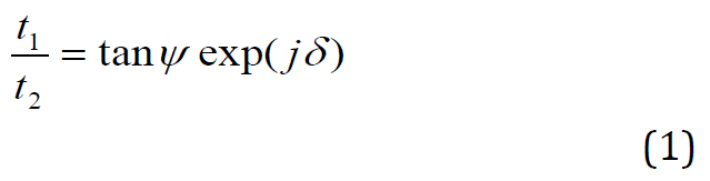
where δ and ψ are ellipsometric parameters respectively related to the difference in phase and magnitude. These two parameters are also related to the birefringence Δn' and the dichroism Δn'' by:
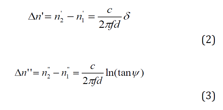
where f is the wave frequency, d the sample’s thickness and c the speed of light.
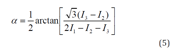
The rotation α (Figure 1) of the major axis of the ellipse referred to the direction of the incident polarization is given by:
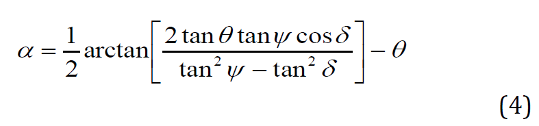
From the measurement of the rotation α for several angular position θ of the sample, it is possible to determine the ellipsometric parameters (δ and ψ) and therefore the anisotropy
of the sample as well as the sample axes.
Experimental Setup
The experimental measurement system (Figure 2) is an ellipsometric workbench made up of a pair of circular horn antennas forming an emitter and a receiver. In between, the measured sample is horizontally placed on a revolving plate actuated by a stepper motor.
The emitter is made of a Gunn source (30 GHz), a rectangular waveguide used as a polarizer and a circular horn antenna with Fresnel lens. The rectangular waveguide polarizes the electric field E of the transmitted wave parallel to its small side. Only the fundamental mode TE10 propagates. The beams are collimated by the Fresnel lens forming a plane wave.
The receiver is also equipped with a circular horn antenna connected to a circular waveguide on which three detectors directed at 120° from each other are perpendicularly connected through portions of rectangular waveguides. Energy is maximal in the detector placed parallel to the direction of the incident polarization. The two other detectors receive the quarter of that energy.
After calibration, the three detectors constitute a set of analyzers, which provides the energy of the electric field in the three directions. From these three values (I1, I2, and I3); we determine the equation of the ellipse and its rotation α.
Figure 2: The Experimental Measurement System
Measurement Technique
The measurement is based on the changes in the polarization of the transmitted (or incident) plane wave through the measured sample.
When rotating, the sample is located by its angular position θ referred to the direction of the incident polarization (Figure 1). The emergent wave is elliptically polarized and its polarization state is determined from the energy values (I1, I2, and I3) of the electric field in the three directions. From these values, we calculate the rotation α of the emerging wave with respect to the initial direction of the transmitted plane wave using Eq. 5.
Applying a numerical least-square analysis to Eq. 4, we can find the ellipsometric parameters (δ and ψ) from which we deduce the index anisotropy Δn in the material through Eq. 2 and Eq. 3.
Sixteen leather samples taken from different part of a calfskin have been measured and analyzed. These samples are in a circle form of diameter varying between 15 and 17 cm with a thickness of 1 to 1.3 mm (Figure 3).
Figure 3: Leather samples
Samples were cut from areas of the skin numbered from 1 to 16 (Figure 4) i.e. from the neck, butt, legs, flanks, and abutment. Their position on the skin is referred to the animal backbone.
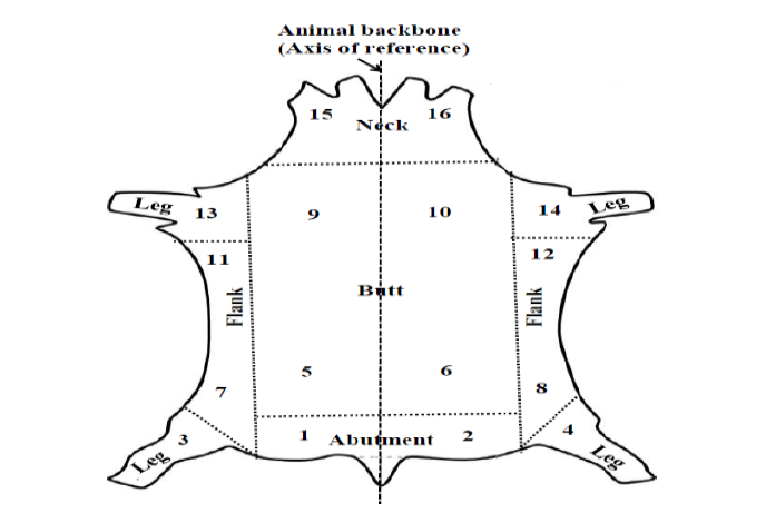
Figure 4: The Calfskin Showing The Different Areas Where the Samples Were Taken. These Areas Are Numbered From 1 To 16
The rotation of the emergent polarization α of the samples is measured by the ellipsometric workbench for different angular positions
In Figure 5, we show the rotations of some few samples.
Figure 5: Rotation of the emergent polarization α (°) against the angular position of the sample θ (°) for some few samples
These rotations can be adjusted using a theoretical curve (Figure 6). Their amplitudes are non-null and lie between 0.5° and 3°.
Figure 6: Example of an Adjustment of the Rotation Α of One of the Samples with a Theoretical Curve In Order To Determine Numerically the Ellipsometric Parameters Δ and Ψ
According to our direct problem, we are here in the case of low amplitudes since samples thickness is very small of about 1 mm. Therefore, the influence of the parameter δ will be less significant and it can take any values between 0° and 10° (i.e.). In this case, we will just consider the influence of ψ (i.e. the dichroism
) which is more significant.
The rotations amplitude of all the samples and their anisotropy are summarized in Table 1.
Table 1: Anisotropy of Leather Samples
| Skin area | Sample | αMax(°) | ψ(°) | Δn’’ | θ0(°) |
| 1 | Left abutment | 0.61 | 45.61 | 0.0338 | -80 |
| 2 | Right abutment | 0.62 | 46.62 | 0.0346 | 70 |
| 3 | Left rear leg | 1.11 | 46.10 | 0.0614 | -25 |
| 4 | Right rear leg | 2.36 | 47.34 | 0.1303 | 30 |
| 5 | Left rear butt | 0.50 | 45.50 | 0.0278 | 0 |
| 6 | Right rear butt | 0.29 | 45.29 | 0.0164 | 25 |
| 7 | Left rear flank | 2.64 | 47.62 | 0.1459 | -10 |
| 8 | Right rear flank | 1.63 | 46.63 | 0.0904 | 5 |
| 9 | Left front butt | 0.43 | 45.42 | 0.0236 | 10 |
| 10 | Right front butt | 0.66 | 45.65 | 0.0364 | 20 |
| 11 | Left front flank | 1.31 | 46.31 | 0.0725 | 0 |
| 12 | Right front flank | 1.49 | 46.41 | 0.0826 | 5 |
| 13 | Left front leg | 1.52 | 46.52 | 0.0847 | 45 |
| 14 | Right front leg | 1.27 | 46.27 | 0.0708 | -30 |
| 15 | Left neck | 2.01 | 47.01 | 0.1117 | 15 |
| 16 | Right neck | 0.54 | 45.54 | 0.0298 | -20 |
The curves in Figure 5 show that some samples have higher rotational amplitude than others and the curves are phase shifted from each other. The amplitudes reflect the anisotropy of the samples and the phase shifts their axes of anisotropy.
From data in Table 1, we have drawn a graph of the anisotropy against the amplitude (Figure 7). The result is a straight line passing through zero which shows proportionality between the amplitude of the sample and its anisotropy. On this line, we clearly distinguish two separate areas, one of low anisotropy and another of high anisotropy, in which we can classify the samples. Therefore, samples from the neck, legs, and flanks have higher anisotropy compared to those of the butt and abutment who are of low anisotropy.
Figure 7: Proportionality between the amplitude of the samples and their anisotropy Δn'
Determination of Samples Axes
The sample axes (known also as neutral axes) are formed by the arrangement of collagen fibers. In Figure 8, when the rotation α equals to zero (α = 0), it means that the transmitted wave has passed through a specific direction which could be one of the neutral axes of the sample. So, resistance to stretching will be minimum or maximum in this direction. Note that neutral axes are always perpendicular to each other. To show that, let’s consider for example the measurement of the right rear leg sample in Figure 8. For α = 0, we find θ0 = 30°. This means that one of the sample axes is at 30° referred to the animal backbone. The second axis is systematically 90° away from the first one (i.e. at 120°), this is clearly shown in Figure 8. The direction of the neutral axes θ0 of the remaining samples referred to the animal backbone is summarized in Table 1.
Figure 8: Direction of the Neutral Axes of the Right Rear Leg Sample Referred To the Animal Backbone
Figure 9 shows schematically the arrangement of the neutral axes according to the different parts of the skin. We can see their deviation from the axis of the animal backbone taken as reference.
This result is consistent with that obtained in previous work [3]. Fibers orientations shown in Figure9 are almost similar to the orientational distribution map of collagen fibers in the whole calfskin presented by Osaki.

Figure 9: Samples Axes Referred To the Animal Backbone
This study has enabled us to demonstrate that it is possible to characterize leather samples using transmission ellipsometry. The study has been carried out even though samples thicknesses were small (in the order of a millimeter) compared to the wavelength of 1 cm. We were able to determine the anisotropy in leather samples which were classified into two groups with respect to their degree of anisotropy. We also clearly determined samples axes relative to areas where they were taken.
Further work on this method might concentrate on the use of multi-frequency transmission measurements in oblique incidence in order to determine the absolute index of the material.
Acknowledgment
I would like to give a special thanks to Cedric VIGIER who supplied leather samples from the CTC- Centre Technique Cuir Chaussure Maroquinerie, of Lyon, France.
Dempsey, M. “The structure of the skin and leather manufacture.” Journal of the Royal Microscopical Society, vol. 67, no. 1–4, 1947, pp. 21–26.
Green, M. et al. “Collagen fiber orientation in bovine secondary osteons by collagenase etching.” Biomaterials, vol. 8, no. 6, 1987, pp. 427–432.
Osaki, S. “Distribution map of collagen fiber orientation in a whole calf skin.” Anatomical Record, vol. 254, no. 1, 1999, pp. 147–152.
Osaki, S. “Use of hair pores to determine the orientation of collagen fibers in skin.” Anatomical Record, vol. 263, no. 2, 2001, pp. 161–166.
Niitsuma, K. et al. “Microwaves determine the orientational distribution of collagen fibers in a whole cobra skin.” Polymer Journal, vol. 39, no. 2, 2007, pp. 181–186.
Gambou, F. et al. “Characterization of material anisotropy using microwave ellipsometry.” Microwave and Optical Technology Letters, vol. 53, no. 9, 2011, pp. 1996–1998.
Gambou, F. et al. “Microwave characterization of Chadian Palmyra wood (Borassus aethiopum).” Scholars Journal of Engineering and Technology, vol. 6, no. 4, 2018, pp. 119–126.
Moungache, A. et al. “Measurement of refraction index of thick and nontransparent isotropic material using transmission microwave ellipsometry.” Microwave and Optical Technology Letters, vol. 57, no. 4, 2015, pp. 1006–1013.
Sagnard, F. et al. “In situ measurements of the complex permittivity of materials using reflection ellipsometry in the microwave band: Theory (part I).” IEEE Transactions on Instrumentation and Measurement, vol. 54, no. 3, 2005a, pp. 1266–1273.
Sagnard, F. et al. “In situ measurements of the complex permittivity of materials using reflection ellipsometry in the microwave band: Experiments (part II).” IEEE Transactions on Instrumentation and Measurement, vol. 54, no. 3, 2005b, pp. 1274–1282.
Azzam, R.M.A. and N.M. Bashara. Ellipsometry and Polarized Light. Elsevier Science, 1987.