In today's visually-driven world, images play a crucial role in conveying information, capturing memories and inspiring emotions. However, the process of capturing and transmitting images is not always perfect, often resulting in the presence of unwanted noise that can degrade the overall quality and clarity of the image. This is where the field of image de-noising comes into play [1,2]. Image de-noising is the process of reducing or eliminating unwanted noise from digital images while preserving essential details and maintaining image integrity. It involves employing various mathematical and computational techniques to distinguish between noise and the actual image content, enhancing the visual experience for viewers. The presence of noise in images can arise from several sources, including sensor limitations, low light conditions, compression artifacts and transmission errors.         

Noise can manifest as random fluctuations in pixel values, leading to a loss of sharpness, increased graininess and decreased visual fidelity [3]. Image de-noising algorithms aim to restore the image to its original quality by minimizing the noise without significantly altering the underlying content. Over the years, significant advancements in image de-noising techniques have been made, driven by the increasing demand for high-quality visual content in fields such as photography, medical imaging [4,5], surveillance [6] and computer vision [7]. From traditional methods like spatial filtering and statistical modelling to more sophisticated approaches like deep learning-based algorithms, researchers continue to explore innovative solutions for effective image de-noising. Image de-noising techniques encompass a wide range of algorithms and methodologies aimed at reducing or eliminating noise from digital images. These techniques leverage advanced mathematical models, statistical analysis and signal processing approaches to distinguish between noise and actual image content, enhancing visual fidelity. Traditional image de-noising techniques [8] include spatial filtering, which involves applying filters to individual pixels or neighborhoods within the image to smooth out noise. Statistical modelling techniques exploit the statistical properties of noise to separate it from the underlying image. These techniques have been widely employed and have laid the foundation for further advancements. In recent years, with the advent of deep learning and the availability of large-scale datasets, new and highly effective image de-noising techniques have emerged. Deep neural networks, particularly Convolutional Neural Networks (CNNs) [9], have revolutionized the field by learning intricate representations of image structures and noise patterns. By training on diverse datasets, these networks can discern noise characteristics and produce de-noised images that exhibit impressive visual quality.

In [10], a new technique was presented to de-noise Magnetic Resonance Imaging (MRI) images by utilizing Non-Local Means (NLM) [11] and non-subsampled Shearlet (NSST). The presented results showed the effectiveness of the proposed approach in de-noising this type of images when compared to other previously suggested approaches. In [12], authors proposed a new image de-noising technique based on an enhanced sparse representation in the transform domain called block-batching and 3-D filtering (BM3D). The technique involved grouping similar Two-Dimensional (2D) image fragments into Three-Dimensional (3D) data arrays and using collaborative filtering, Wiener Filters [13], to attenuate noise and reveal fine details while preserving unique features. In [14], an attention-guided de-noising convolutional neural network (AD-Net) as an image de-noising technique was proposed. It included a sparse block, a feature enhancement block, an attention block and a reconstruction block to remove noise from images effectively. That paper used synthetic and real noisy images for testing the proposed ADNet model's performance in three tasks, including synthetic and real noisy images and blind de-noising. In [15], a filter based on the Wiener filter and the high-boost filter for medical images was presented. The proposed filter was applied to the degraded image. First, the degraded image and the high-boost filter were converted in the frequency domain using Fourier Transform. Then, the image was processed with the Wiener and the high-boost filters. Finally, the deconvolution process was performed on the image using the high-boost filter. The final step involves taking the inverse of the Fourier transformation was applied to reconstruct a sharper image in the spatial domain. The proposed filter worked to suppress the additive noise while preserving the edge details of the image. To test the effectiveness of the proposed algorithm, focus operators such as image contrast, gradient energy, histogram entropy and spatial frequency were utilized. Experimental results demonstrated that the proposed filter yielded superior outcomes compared to traditional filters, particularly for dark medical images. In [16], the limitations of discriminative learning methods that require multiple models for de-noising images with different noise levels and lack flexibility to deal with spatially variant noise was discussed. In order to address these issues, that paper proposed a fast and flexible de-noising convolutional neural network called FFDNet, which takes a tunable noise level map as input and works on down-sampled sub-images. The proposed FFDNet showed several desirable properties, including the ability to handle a wide range of noise levels effectively with a single network, the ability to remove spatially variant noise by specifying a non-uniform noise level map. The paper concluded by stating that extensive experiments on synthetic and real noisy images are conducted to evaluate FFDNet in comparison with state-of-the-art de-noising techniques and the results show that FFDNet was effective and efficient, making it highly attractive for practical de-noising applications. In [17], a new hybrid system for image de-noising was proposed. It utilizes BM3D algorithm to obtain an initial de-noised image. Then, the weighted kernel Norm Minimization (WNNM) and NSST algorithms are applied successively to obtain a second de-noised image. To enhance the details of the second de-noised image, texture information from the first de-noised image is extracted using gradient domain guided filtering. The proposed adaptive iterative NSST algorithm, which improves soft limiting, addresses issues related to the hard limiting discontinuity and the constant deviation of the soft limiting. Their approach not only reduced excessive smoothing but also restored the image's natural appearance. Experimental results demonstrated that that method outperformed several Deep learning de-noising methods. In [18], the development of feed-forward de-noising convolutional neural networks (DnCNNs) to incorporate advancements in deep architecture, learning algorithms and regularization methods for image de-noising was presented. Specifically, residual learning and batch normalization techniques were employed to accelerate the training process and enhance de-noising performance. Unlike previously reported discriminative de-noising models that were typically trained for specific noise levels, often focusing on additive white Gaussian noise, their DnCNN model can handle Gaussian de-noising with unknown noise levels (blind Gaussian de-noising). Through the residual learning approach, DnCNN implicitly eliminates the latent clean image within its hidden layers. This characteristic was the motivation to train a single DnCNN model capable of handling various image de-noising tasks, such as Gaussian de-noising, single image super-resolution and JPEG image deblocking. That paper contained extensive experiments that demonstrate that the DnCNN model not only exhibits remarkable effectiveness in various image denoising tasks but also efficiently leverages Graphics Processing Unit (GPU) computing for implementation.

In this work, a de-noising approach is proposed that incorporates an adaptive algorithm to preserve specific number of Cosine coefficients. Such coefficients are selected based on a data-driven threshold, resulting in a less noisy image for Additive White Gaussian Noise (AWGN). The adaptive algorithm iteratively decomposes the noisy image into the Cosine and the Haar domains, until an energy-based predefined limit is reached. The proposed approach is evaluated using publicly available grayscale images and compared against state-of-the-art systems. Peak Signal to Noise Ratio (PSNR) is used as a metric, along with visual inspection by human observer. The results demonstrate that the proposed system outperforms the compared system in terms of the metrics used.

EXPERIMENTAL PROGRAM

Adaptive Coefficients Selection Algorithm

The adaptive coefficients selection algorithm, shown in Figure 1, is implemented in the following manner [19]. The input image is converted the Cosine domain using the appropriate transform formula. Number of coefficients are retained, based on their relatively high content of energy and the rest of the coefficients are sent back to the original domain using the formula for the inverse transform. Then, the Haar function is utilized to transform the signal from the previous step. Also, few coefficients are retained while the rest are converted back to the time domain. The energy left, i.e., the residual, in the time domain is calculated and compared with a predefined limit. The above procedure is repeated until the residual energy falls bellow 0.5% of the original image energy. The final output of the algorithm is 2 two-dimensional weight matrices, one for each domain and the weights range is [0, 1]. Each weight, in each matrix, is the weight of the coefficient in same exact location in the transform coefficients matrix.

Proposed Scheme 

The proposed scheme is shown in Figure 2. The AWGN, with a specific energy level, is added to the clean grey scale image to produce the noisy image. Then, the noisy image is analyzed using the adaptive algorithm explained in section 2.1. Only Cosine coefficients that have weights that exceed the average of all weights are selected and the rest of the coefficients are set to zero. The resultant data matrix is transformed back to the time domain using the Inverse Cosine transform to produce the de-noised image.

The metric utilized in this work to show the effectiveness of the proposed technique is the Peak Signal to Noise Ratio calculated as follows:

                                                      (1)

where, R=255 for grey-scale image and Mean Squared Error (MSE) is calculated as follows:

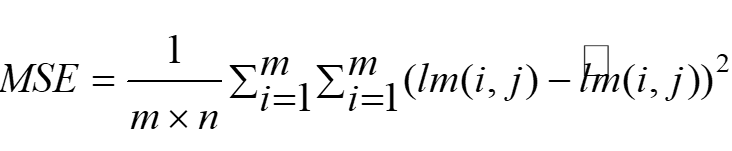
                                     (2)

where, m and n are the image dimensions. The original image is represented in Eq. (2) as Im while (lm) represents the modified image (for this work it is the resultant de-noised image).

The proposed system is tested with publically available images shown in Figure 3. The results are shown in Figure 4 for the case when AWGN variance is 0.03. To have a fair comparison with the most recent reported results of other techniques, the following parameters were considered when implementing the proposed technique. Images 1 through 7 were 256*256 grey scale images. On the other hand, images 8 through 12 are set to 512*512. The AWGN variances were: 0.01, 0.03 and 0.05 respectively.

Tables 1 through 3 show all results obtained for the proposed techniques with results reported in other references. The results shown in the tables, they are the differences between the maximum obtained PSNR for each image and the PSNR obtained for that technique, are either zero or negative real number. The zeros represent the maximum obtained PSNRs for that image, column wise and hence the negative numbers mean less PSNR.

Figure 1: Adaptive Algorithm in Two Domains, Cosine and Haar

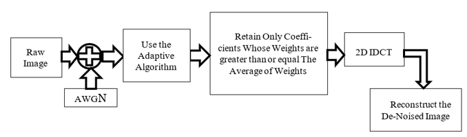
Figure 2: Proposed Scheme to De-Noise Images Based on The Adaptive Algorithm

Table 1: Relative PSNR for the Proposed Scheme and Other Recently Reported De-Noising Techniques, where 0.00 refers to the maximum obtained PSNR while the rest are the relative decrease PSNR obtained for the Same Image. I1 is the first image; I2 is the second, etc.

Table 2: Relative PSNR for the Proposed Scheme and Other Recently Reported De-Noising Techniques, where 0.00 refers to the maximum obtained PSNR while the rest are the relative decrease PSNR obtained for the Same Image. I1 is the first image; I2 is the second, etc.

Table 3: Relative PSNR for the Proposed Scheme and Other Recently Reported De-Noising Techniques, where 0.00 refers to the maximum obtained PSNR while the rest are the relative decrease PSNR obtained for the Same Image. I1 is the first image; I2 is the second, etc.

Figure 3: Publically Available Images Utilized To Test the Proposed Scheme. Images are ordered 1 to 12 starting left/right then up/down

Figure 4: Results of Applying the Proposed Scheme Along with Other Recently Reported Techniques on Publically Available Images (AWGN =0.03)

As shown in Tables 1 through 3, the proposed scheme outperformed the other techniques (on average) for AWGN variances 0.03 and 0.05. The first case, variance is 0.01, the proposed scheme was -0.12 dB away (on average) from the best-reported technique. The last case, variance is 0.05, the proposed scheme outperforms other techniques on average and for each individual image.

In addition, de-noised images using proposed scheme has a comparable visual quality with images obtained from other reported techniques as shown in Figure 4.

In this work, a new grey scale image de-noising scheme based on Cosine coefficients is proposed. The selection of such coefficients is based on their weights. Such weights are computed through an iterative algorithm utilized to analyze the noisy images in two domains, namely, Cosine and Haar. The results obtained for the proposed technique are compared with recently reported de-noising techniques for the same images and same noise variance levels. As shown in the comparison, the proposed work performs better in terms of PSNR than the rest of the techniques. In addition, the visual quality of the de-noised images using the proposed work is equal or better when compared with those techniques.

1. Lakshmi, Rama, Gali G., Divya D., Bhavya D., Sai Jahnavi Ch and Akila B. "A review on image denoising algorithms for various applications." Proceedings of Fourth International Conference on Communication, Computing and Electronics Systems: ICCCES 2022, Springer Nature Singapore, 2023, pp. 839–847.

2. Singh, A., Kushwaha S., Alarfaj M. and Singh M. "Comprehensive overview of backpropagation algorithm for digital image denoising." Electronics, vol. 11, no. 10, May 2022, p. 1590.

3. Izadi, S., Sutton D. and Hamarneh G. "Image denoising in the deep learning era." Artificial Intelligence Review, vol. 56, 2023, pp. 5929–5974, https://doi.org/10.1007/s10462-022-10305-2.

4. Kaur, A. and Dong G. "A complete review on image denoising techniques for medical images." Neural Processing Letters, 4 July 2023, pp. 1–44, https://doi.org/10.1007/s11063-023-11286-1.

5. Patil, R. and Bhosale S. "Medical image denoising techniques: a review." International Journal on Engineering, Science and Technology (IJonEST), vol. 4, no. 1, 17 Jan. 2022, pp. 21–33, https://doi.org/10.46328/ijonest.76.

6. Domingos, L.C. et al. "A survey of underwater acoustic data classification methods using deep learning for shoreline surveillance." Sensors, vol. 22, no. 6, Mar. 2022, p. 2181, https://doi.org/10.3390/s22062181.

7. Li, R. et al. "Research on the application status of machine vision technology in furniture manufacturing process." Applied Sciences, vol. 13, no. 4, 2023, p. 2434, https://doi.org/10.3390/app13042434.

8. Abedini, M. et al. "Image denoising using sparse representation and principal component analysis." International Journal of Image and Graphics, vol. 22, no. 4, 17 July 2022, p. 2250033, https://doi.org/10.1142/S0219467822500334.

9. Zhang, Q. et al. "Hyperspectral image denoising: from model-driven, data-driven, to model-data-driven." IEEE Transactions on Neural Networks and Learning Systems, 6 June 2023, https://doi.org/10.1109/TNNLS.2023.3278866.

10. Sharma, A. and Chaurasia V. "MRI denoising using advanced NLM filtering with non-subsampled shearlet transform." Signal, Image and Video Processing, vol. 15, Sept. 2021, pp. 1331–39, https://doi.org/10.1007/s11760-021-01864-y.

11. Manjón, J.V. et al. "MRI denoising using non-local means." Medical Image Analysis, vol. 12, no. 4, 1 Aug. 2008, pp. 514–23, https://doi.org/10.1016/j.media.2008.02.004.

12. Dabov, K., et al. "Image denoising by sparse 3-D transform-domain collaborative filtering." IEEE Transactions on Image Processing, vol. 16, no. 8, 16 July 2007, pp. 2080–95, https://doi.org/10.1109/TIP.2007.901238.

13. Zhang, Q. et al. "An improved Wiener filter based on adaptive SNR MRI image denoising algorithm." 2022 International Conference on Computing, Communication, Perception and Quantum Technology (CCPQT), 5 Aug. 2022, pp. 164–68, https://doi.org/10.1109/CCPQT56151.2022.00036.

14. Tian, C. et al. "Attention-guided CNN for image denoising." Neural Networks, vol. 124, Apr. 2020, pp. 117–29, https://doi.org/10.1016/j.neunet.2019.12.024.

15. Habeeb, N.J. "Medical image denoising with Wiener filter and high boost filtering." Iraqi Journal of Science, vol. 64, no. 6, 30 June 2023, pp. 4023–35, https://doi.org/10.24996/ijs.2023.64.6.40.

16. Zhang, K. et al. "FFDNet: Toward a fast and flexible solution for CNN-based image denoising." IEEE Transactions on Image Processing, vol. 27, no. 9, 25 May 2018, pp. 4608–22, https://doi.org/10.1109/TIP.2018.2839891.

17. Li, Z., Liu H. et al. "Image denoising algorithm based on gradient domain guided filtering and NSST." IEEE Access, vol. 11, 3 Feb. 2023, pp. 11923–33, https://doi.org/10.1109/ACCESS.2023.3242050.

18. Zhang, K. et al. "Beyond a Gaussian denoiser: Residual learning of deep CNN for image denoising." IEEE Transactions on Image Processing, vol. 26, no. 7, 1 Feb. 2017, pp. 3142–55, https://doi.org/10.1109/TIP.2017.2662206.

19. Ramaswamy, A. and Mikhael W.B. "Multitransform/multidimensional signal representation." Proceedings of 36th IEEE Midwest Symposium on Circuits and Systems, 16 Aug. 1993, pp. 1255–58, https://doi.org/10.1109/MWSCAS.1993.343326.